2.2 Unipart network for seed lots analysis
This section deals with unipart network that represents the relationships between seed lots.
2.2.1 Steps with PPBstats
- Format the data with
format_data_PPBstats() - get descriptive plot with
plot()
2.2.2 Format the data
The format required is a data frame with the following compulsory columns as factor:
"seed_lot_parent": name of the parent seed lot in the relationship"seed_lot_child"; name of the child seed lots in the relationship"relation_type": the type of relationship between the seed lots"relation_year_start": the year when the relationship starts"relation_year_end": the year when the relationship stops"germplasm_parent": the germplasm associated to the parent seed lot"location_parent": the location associated to the parent seed lot"year_parent": the year of the last relationship of the parent seed lot"germplasm_child": the germplasm associated to the child seed lot"location_child": the location associated to the child seed lot"year_child": represents the year of the last relation event of the child seed lot
Possible options are : "long_parent", "lat_parent", "long_child", "lat_child" to get map representation, supplementary variables with tags: "_parent", "_child" or "_relation".
The format of the data are checked by the function format_data_PPBstats() with the following arguments :
type:"data_network"network_part:"unipart"vertex_type:"seed_lots"
The function returns list of igraph object1 coming from igraph::graph_from_data_frame().
data(data_network_unipart_sl)
head(data_network_unipart_sl)
## seed_lot_parent seed_lot_child relation_type
## 1 germ-8_loc-1_2007_0001 germ-8_loc-1_2008_0001 selection
## 2 germ-8_loc-1_2008_0001 germ-8_loc-1_2009_0001 reproduction
## 3 germ-8_loc-1_2009_0001 germ-8_loc-2_2009_0001 diffusion
## 4 germ-8_loc-1_2008_0001 germ-8_loc-1_2009_0001 selection
## 5 germ-1_loc-1_2005_0001 germ-8_loc-1_2006_0001 reproduction
## 6 germ-6_loc-1_2005_0001 germ-8_loc-1_2006_0001 reproduction
## relation_year_start relation_year_end germplasm_parent location_parent
## 1 2007 2008 germ-8 loc-1
## 2 2008 2009 germ-8 loc-1
## 3 2009 2009 germ-8 loc-1
## 4 2008 2009 germ-8 loc-1
## 5 2005 2006 germ-1 loc-1
## 6 2005 2006 germ-6 loc-1
## year_parent alt_parent long_parent lat_parent germplasm_child
## 1 2007 50 0.616363 44.20314 germ-8
## 2 2008 50 0.616363 44.20314 germ-8
## 3 2009 50 0.616363 44.20314 germ-8
## 4 2008 50 0.616363 44.20314 germ-8
## 5 2005 50 0.616363 44.20314 germ-8
## 6 2005 50 0.616363 44.20314 germ-8
## location_child year_child alt_child long_child lat_child
## 1 loc-1 2008 50 0.616363 44.20314
## 2 loc-1 2009 50 0.616363 44.20314
## 3 loc-2 2009 360 3.087025 45.77722
## 4 loc-1 2009 50 0.616363 44.20314
## 5 loc-1 2006 50 0.616363 44.20314
## 6 loc-1 2006 50 0.616363 44.20314net_unipart_sl = format_data_PPBstats(
type = "data_network",
data = data_network_unipart_sl,
network_part = "unipart",
vertex_type = "seed_lots")## data has been formated for PPBstats functions.length(net_unipart_sl)## [1] 1head(net_unipart_sl)## [[1]]
## IGRAPH 874b15c DN-- 81 94 --
## + attr: name (v/c), germplasm (v/c), location (v/c), year (v/c),
## | alt (v/c), long (v/c), lat (v/c), format (v/c), relation_type
## | (e/c)
## + edges from 874b15c (vertex names):
## [1] germ-8_loc-1_2007_0001->germ-8_loc-1_2008_0001
## [2] germ-8_loc-1_2008_0001->germ-8_loc-1_2009_0001
## [3] germ-8_loc-1_2009_0001->germ-8_loc-2_2009_0001
## [4] germ-8_loc-1_2008_0001->germ-8_loc-1_2009_0001
## [5] germ-1_loc-1_2005_0001->germ-8_loc-1_2006_0001
## [6] germ-6_loc-1_2005_0001->germ-8_loc-1_2006_0001
## + ... omitted several edges2.2.3 Describe the data
The different representations are done with the plot() function.
For network representation, set plot_type = "network" diffusion event are displayed with a curve.
in_col can be settled to customize color of vertex.
p_net = plot(net_unipart_sl, plot_type = "network", in_col = "location")
p_net
## [[1]]
## [[1]]$network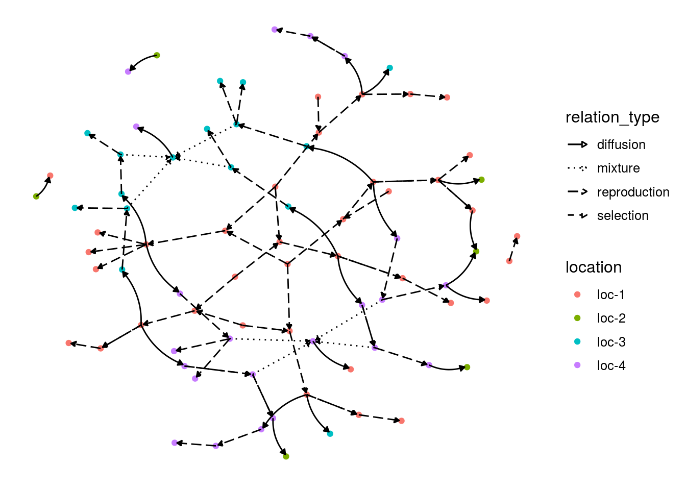
In order to get the network organized in a chronologiical order and by location, set organize_sl = TRUE.
This representation is possible if the seed lots are under the following format : GERMPLASM_LOCATION_YEAR_DIGIT.
p_net_org = plot(net_unipart_sl, plot_type = "network", organize_sl = TRUE)
p_net_org
## [[1]]
## [[1]]$network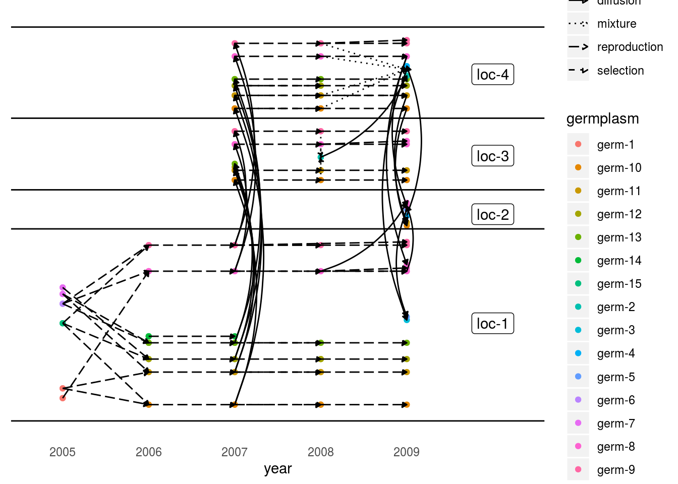
To have information on the seed lots that are represented, plot_type = "barplot" can be used.
Choose what to represent on the x axis and in color as well as the number of parameter per plot.
p_bar = plot(net_unipart_sl, plot_type = "barplot", in_col = "location",
                          x_axis = "germplasm", nb_parameters_per_plot_x_axis = 5,
                          nb_parameters_per_plot_in_col = 5)
p_bar[[1]]$barplot$`germplasm-1|location-1` # first element of the plot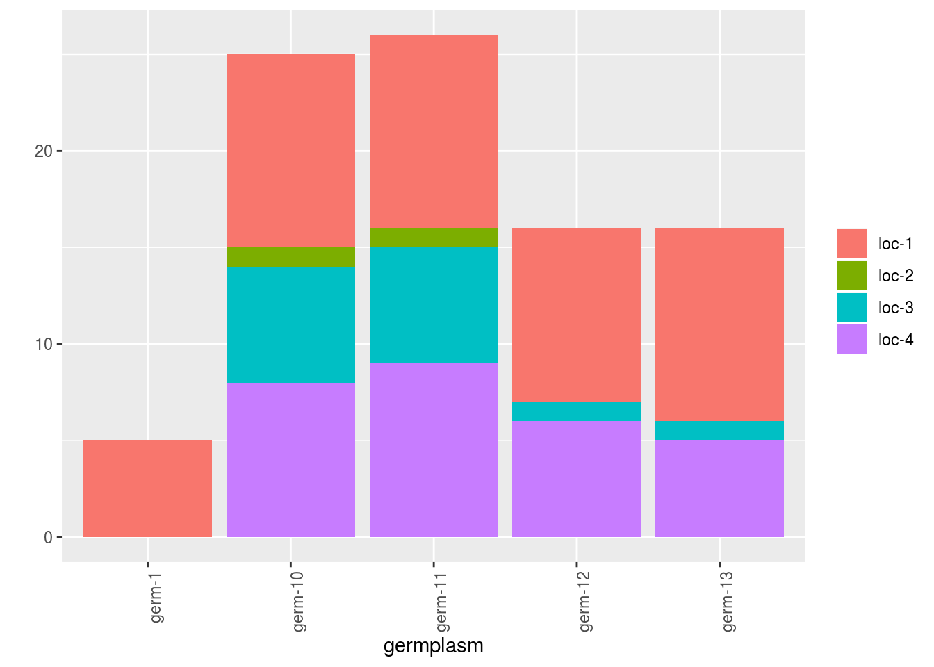
Barplot can also be use to study the relation within the network.
The name of the relation must be put in the argument vec_variables.
The results is a list of two elements for each variable:
- nb_received: number of seed lots that end the relation
- nb_given: number of seed lots that start the relation
p_bar = plot(net_unipart_sl, plot_type = "barplot", vec_variables = "diffusion",
                  nb_parameters_per_plot_x_axis = 100, x_axis = "location", in_col = "year")
p_bar
## [[1]]
## [[1]]$diffusion
## [[1]]$diffusion$nb_received
## [[1]]$diffusion$nb_received$`location-1|year-1`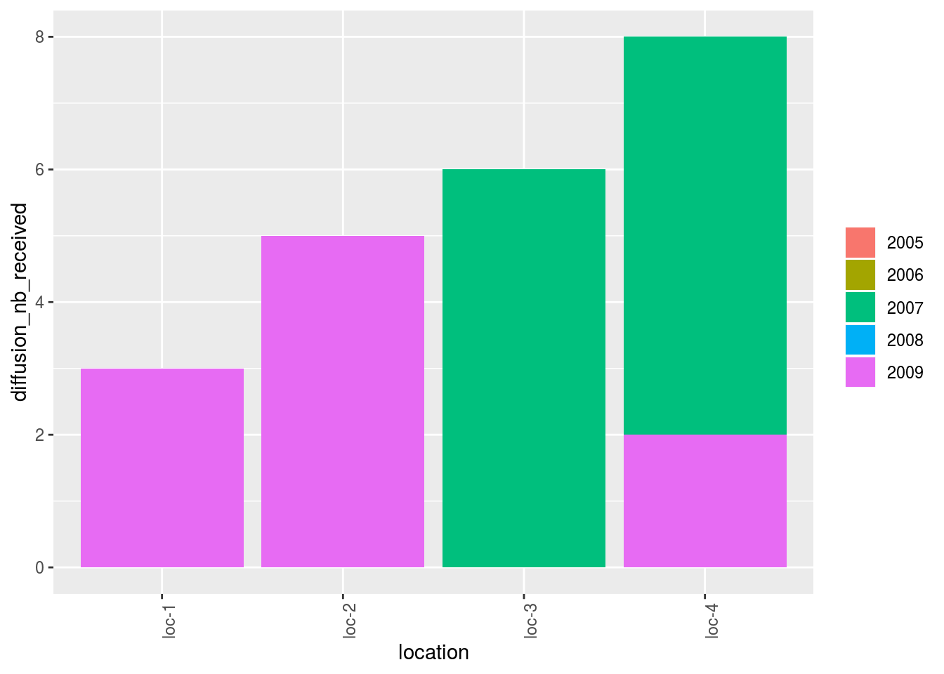
##
##
## [[1]]$diffusion$nb_given
## [[1]]$diffusion$nb_given$`location-1|year-1`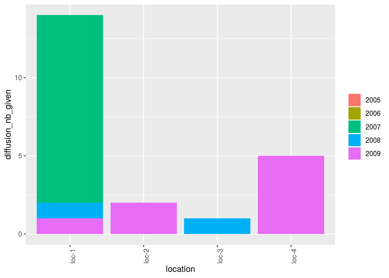
Location present on the network can be displayed on a map with plot_type = "map".
When using map, do not forget to use credit :
Map tiles by Stamen Design,
under CC BY 3.0.
Data by OpenStreetMap,
under ODbL.
p_map = plot(net_unipart_sl, plot_type = "map", labels_on = "location")
p_map
## [[1]]
## [[1]]$map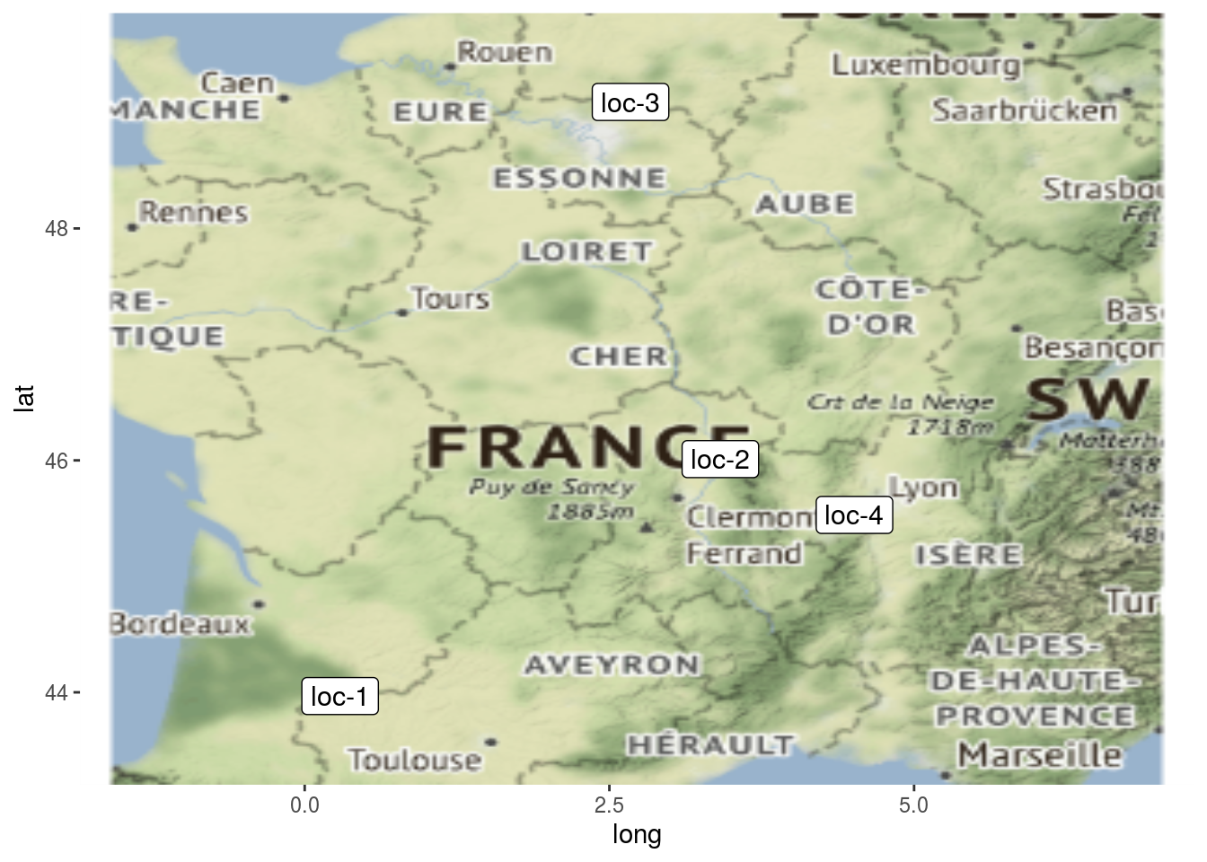
It can be interesting to plot information regarding a variable on map with a pie with plot_type = "map" and by setting arguments data_to_pie and variable:
nb_values = 30
data_to_pie = data.frame(
  seed_lot = rep(c("germ-4_loc-4_2009_0001", "germ-9_loc-4_2009_0001", "germ-10_loc-3_2009_0001", "germ-12_loc-3_2007_0001", "germ-11_loc-2_2009_0001", "germ-10_loc-2_2009_0001"), each = nb_values),
  location = rep(c("loc-1", "loc-1", "loc-3", "loc-3", "loc-2", "loc-2"), each = nb_values),
  year = rep(c("2009", "2008", "2007", "2007", "2009", "2009"), each = nb_values),
  germplasm = rep(c("germ-7", "germ-2", "germ-6", "germ-4", "germ-5", "germ-13"), each = nb_values),
  block = 1,
  X = 1,
  Y = 1,
  y1 = rnorm(nb_values*6, 10, 2), # quanti
  y2 = rep(c("cat1", "cat1", "cat2", "cat3", "cat3", "cat4"), each = nb_values)  # quali
)

data_to_pie$seed_lot = as.factor(as.character(data_to_pie$seed_lot))
data_to_pie$location = as.factor(as.character(data_to_pie$location))
data_to_pie$year = as.factor(as.character(data_to_pie$year))
data_to_pie$germplasm = as.factor(as.character(data_to_pie$germplasm))
data_to_pie$block = as.factor(as.character(data_to_pie$block))
data_to_pie$X = as.factor(as.character(data_to_pie$X))
data_to_pie$Y = as.factor(as.character(data_to_pie$Y))

data_to_pie = format_data_PPBstats(data_to_pie, type = "data_agro")
## data has been formated for PPBstats functions.# y1 is a quantitative variable
p_map_pies_y1 = plot(net_unipart_sl, data_to_pie, plot_type = "map", vec_variables = "y1")
p_map_pies_y1## [[1]]
## [[1]]$y1_map_with_pies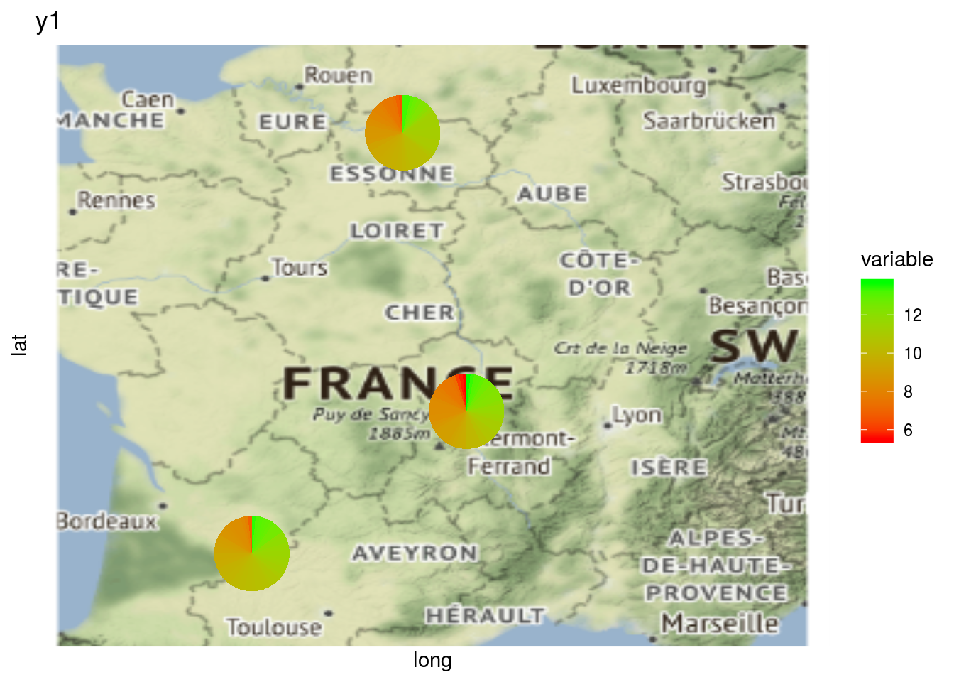
# y2 is a qualitative variable
p_map_pies_y2 = plot(net_unipart_sl, data_to_pie, plot_type = "map", vec_variables = "y2")
p_map_pies_y2
## [[1]]
## [[1]]$y2_map_with_pies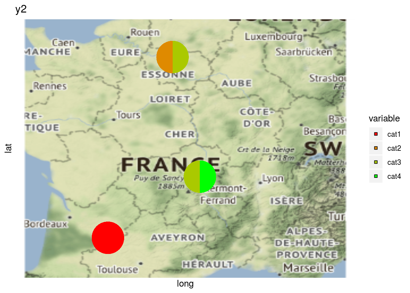
or on the network with a pie with plot_type = "network" and by setting arguments data_to_pie and vec_variables:
# y1 is a quantitative variable
p_net_pies_y1 = plot(net_unipart_sl, data_to_pie, plot_type = "network", vec_variables = "y1")
p_net_pies_y1
## [[1]]
## [[1]]$y1_network_with_pies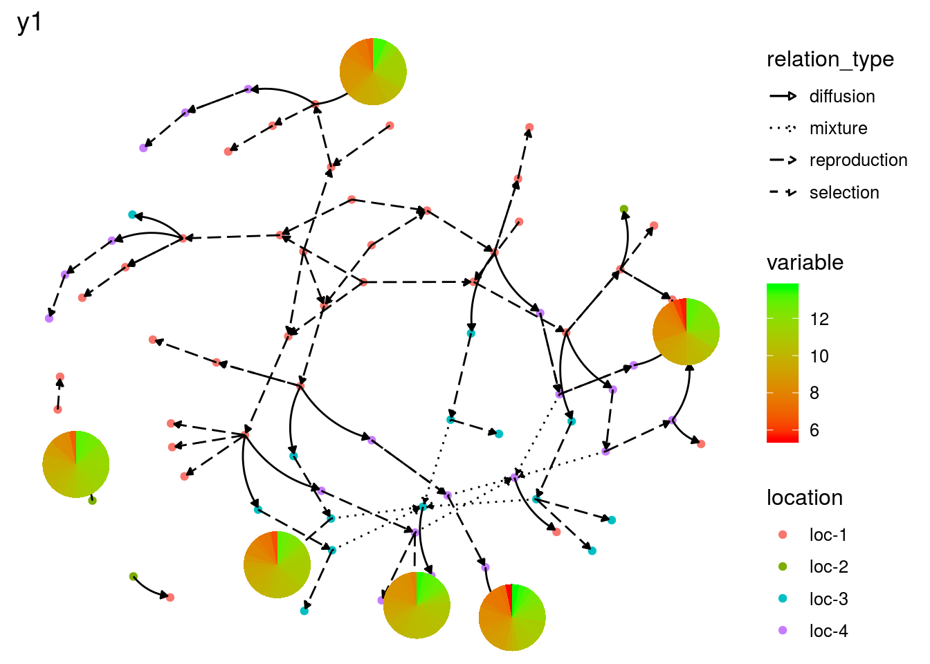
# y2 is a qualitative variable
p_net_pies_y2 = plot(net_unipart_sl, data_to_pie, plot_type = "network", vec_variables = "y2")
p_net_pies_y2
## [[1]]
## [[1]]$y2_network_with_pies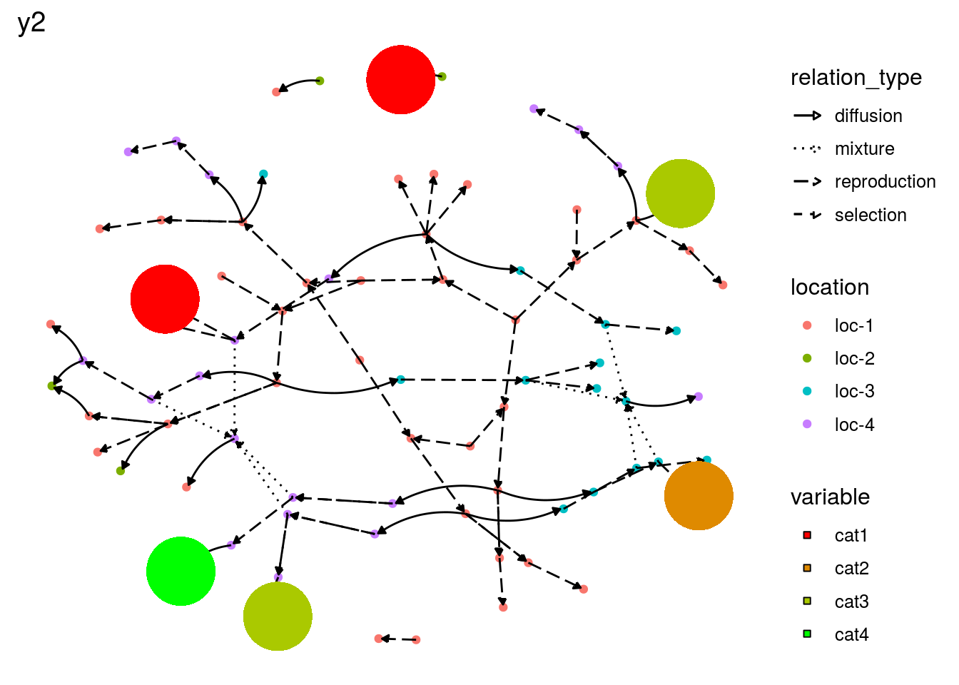
The same can be done regarding relation type of the network. This can be displayed on a map but not on a network.
p_map_pies_diff = plot(net_unipart_sl, plot_type = "map", vec_variables = "diffusion")
p_map_pies_diff
## [[1]]
## [[1]]$diffusion_nb_received_map_with_pies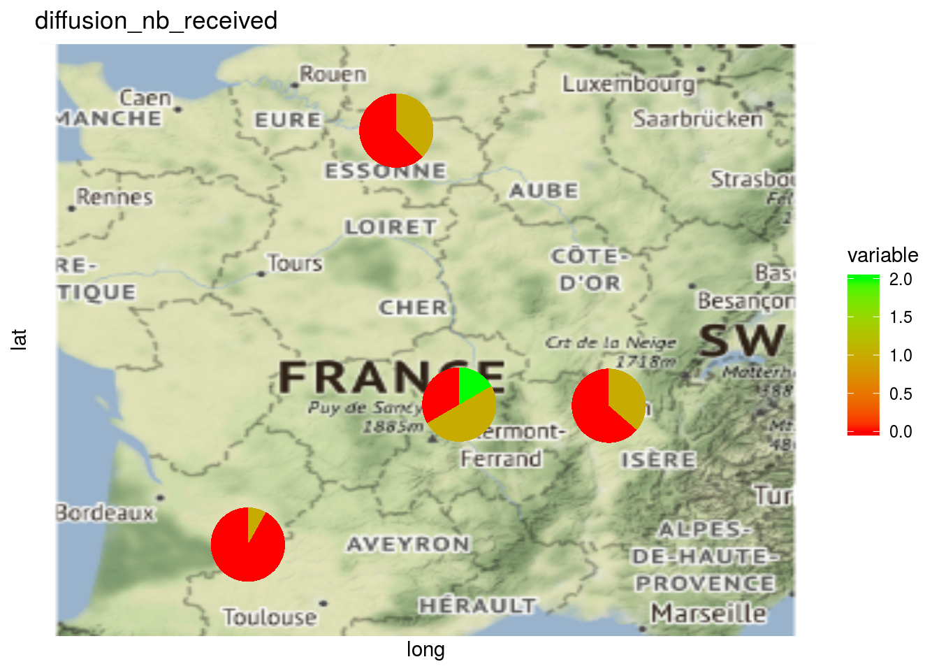
##
## [[1]]$diffusion_nb_given_map_with_pies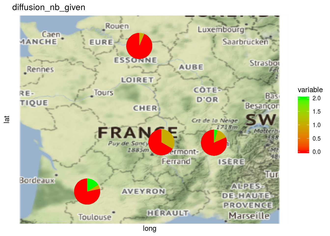
Here the pies represent the repartition of the number of seed lots.