3.4 Describe the data

Once the data have been collected, a first step is to describe them with plot(). Seven types of plot, through the plot_type argument are possible:

• presence abscence matrix that represent the combinaison of germplasm \(\times\) location
• histogramm
• barplot, where sd error are displayed
• boxplot
• interaction
• biplot
• radar
• raster
• map

Then you must choose which factor to represent on the x axis (x_axis argument), the factor to display in color (in_col argument), and of course the variables to describe (vec_variables argument).

It is possible to tune the number of factor displayed (nb_parameters_per_plot_x_axis and nb_parameters_per_plot_in_col arguments) and the size of the labels regarding biplot and radar (labels_on and labels_size arguments).

Note that descriptive plots can be done based on version within the data set. See section 3.8 formore details.

3.4.1 Format the data

Get two data set to look at some examples

data("data_model_GxE")
data_model_GxE = format_data_PPBstats(data_model_GxE, type = "data_agro")

## data has been formated for PPBstats functions.

data("data_model_bh_GxE")
data_model_bh_GxE = format_data_PPBstats(data_model_bh_GxE, type = "data_agro")

## Warning in format_data_PPBstats.data_agro(data): Column "long" is needed to
## get map and not present in data.

## Warning in format_data_PPBstats.data_agro(data): Column "lat" is needed to
## get map and not present in data.

## data has been formated for PPBstats functions.

3.4.2 presence abscence matrix

The presence absence matrix may be different from experimental design planned because of NA. The plot represents the presence/absence matrix of G \(\times\) E combinations.

p = plot(
  data_model_GxE, plot_type = "pam",
  vec_variables = c("y1", "y2")
  )
names(p)

## [1] "y1" "y2"

p$y1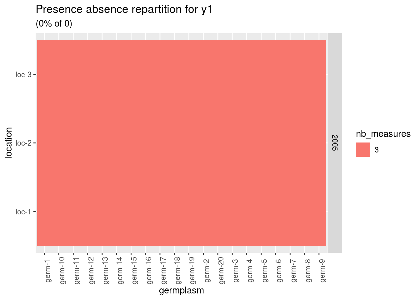

A score of 3 is for a given germplasm replicated three times in a given environement.

p = plot(
  data_model_bh_GxE, plot_type = "pam",
  vec_variables = c("y1", "y2")
  )
p$y1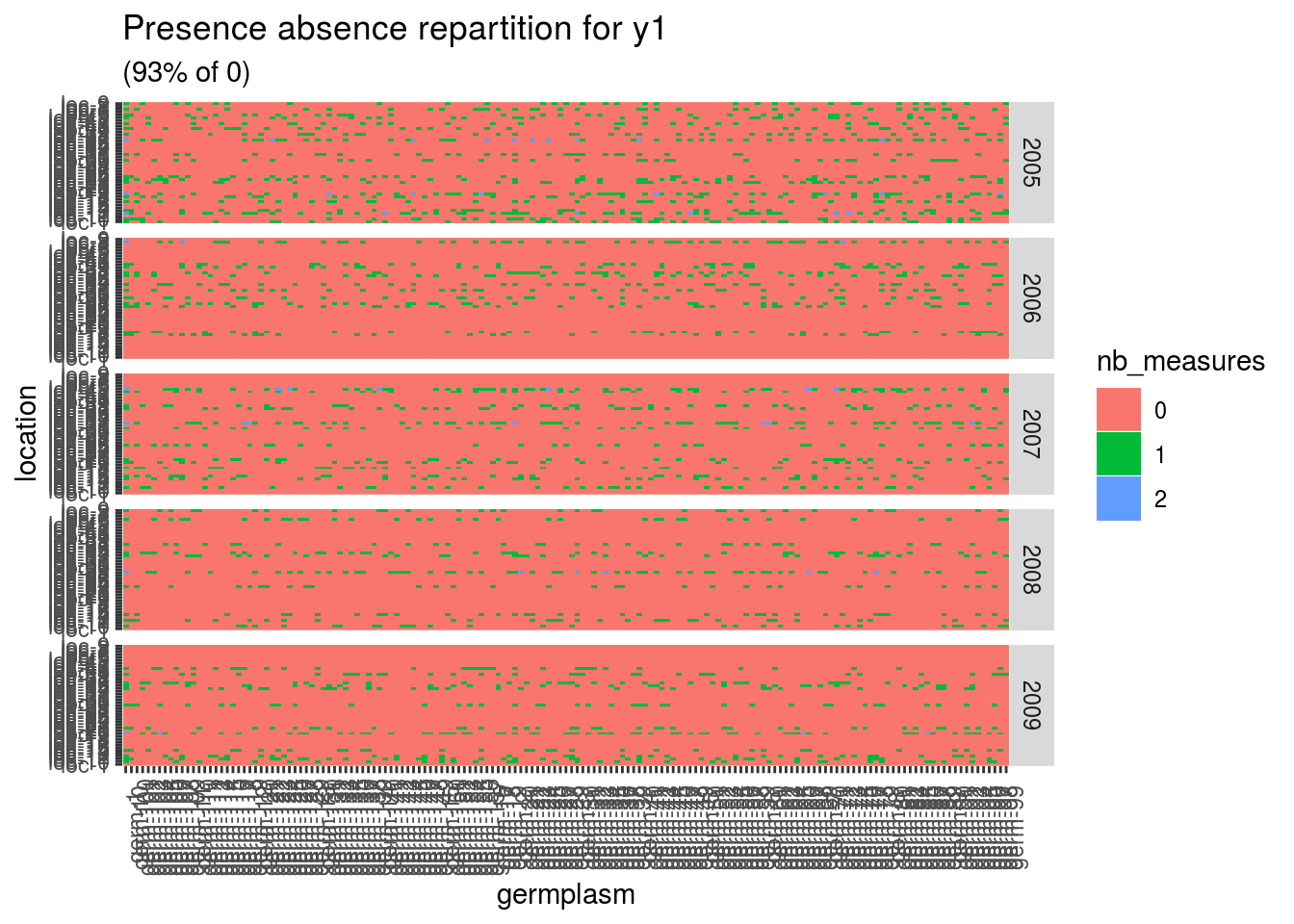

Here there are lots of 0 meaning that a lot of germplasm are no in at least two locations. A score of 1 is for a given germplasm in a given location. A score of 2 is for a given germplasm replicated twice in a given location.

3.4.3 histogramm

p = plot(
  data_model_GxE, plot_type = "histogramm",
  vec_variables = c("y1", "y2")
  )
p$y1

## $`-NA|-NA`

## `stat_bin()` using `bins = 30`. Pick better value with `binwidth`.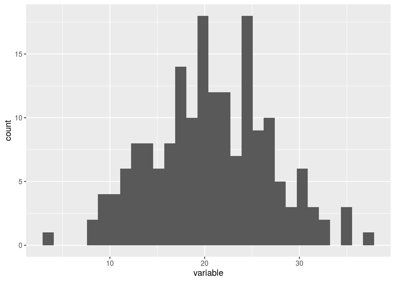

3.4.4 barplot

p = plot(
  data_model_GxE, plot_type = "barplot",
  vec_variables = c("y1", "y2"),
  x_axis = "germplasm"
  )

Note that for each element of the following list, there are as many graph as needed with nb_parameters_per_x_axis parameters per graph.

names(p$y1)

## [1] "germplasm-1|-NA" "germplasm-2|-NA" "germplasm-3|-NA" "germplasm-4|-NA"

p$y1$`germplasm-1|-NA`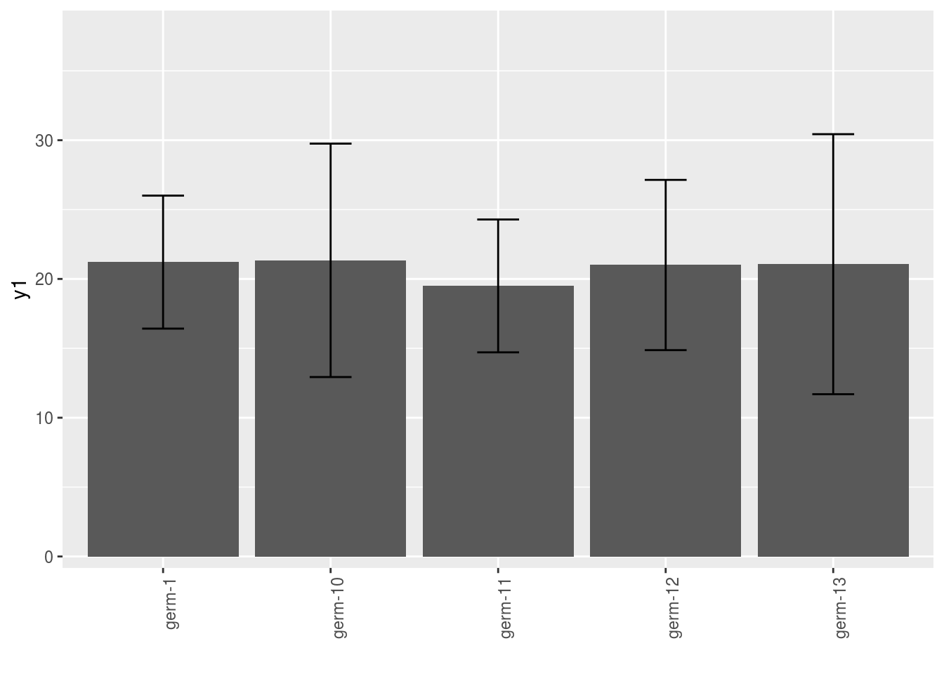

p = plot(
  data_model_GxE, plot_type = "barplot",
  vec_variables = c("y1", "y2"),
  x_axis = "germplasm",
  in_col = "location"
  )

Note that for each element of the following list, there are as many graph as needed with nb_parameters_per_x_axis and nb_parameters_per_in_col parameters per graph.

names(p$y1)

## [1] "germplasm-1|location-1" "germplasm-2|location-1"
## [3] "germplasm-3|location-1" "germplasm-4|location-1"

p$y1$`germplasm-1|location-1`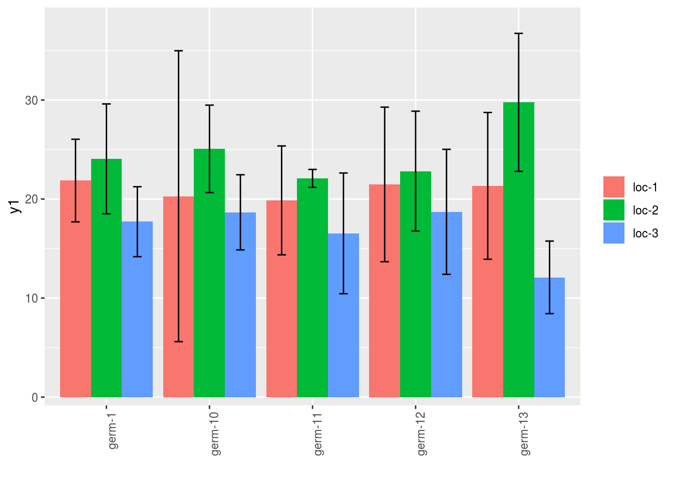

3.4.5 boxplot

p = plot(
  data_model_GxE, plot_type = "boxplot",
  vec_variables = c("y1", "y2"),
  x_axis = "germplasm"
  )

Note that for each element of the following list, there are as many graph as needed with nb_parameters_per_x_axis parameters per graph.

names(p$y1)

## [1] "germplasm-1|-NA" "germplasm-2|-NA" "germplasm-3|-NA" "germplasm-4|-NA"

p$y1$`germplasm-1|-NA`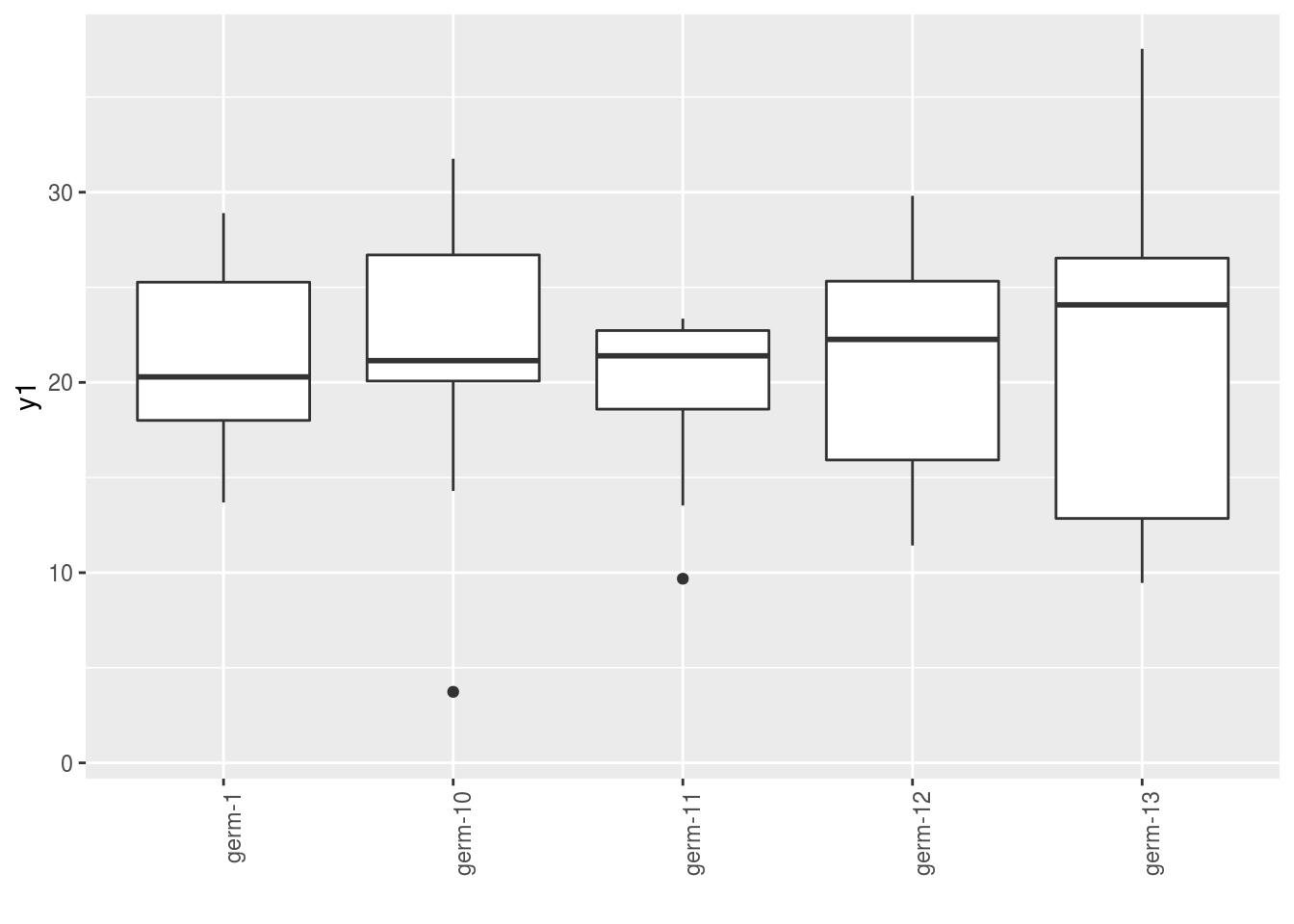

p = plot(
  data_model_GxE, plot_type = "boxplot",
  vec_variables = c("y1", "y2"),
  x_axis = "germplasm",
  in_col = "location"
  )

Note that for each element of the following list, there are as many graph as needed with nb_parameters_per_x_axis and nb_parameters_per_in_col parameters per graph.

names(p$y1)

## [1] "germplasm-1|location-1" "germplasm-2|location-1"
## [3] "germplasm-3|location-1" "germplasm-4|location-1"

p$y1$`germplasm-1|location-1`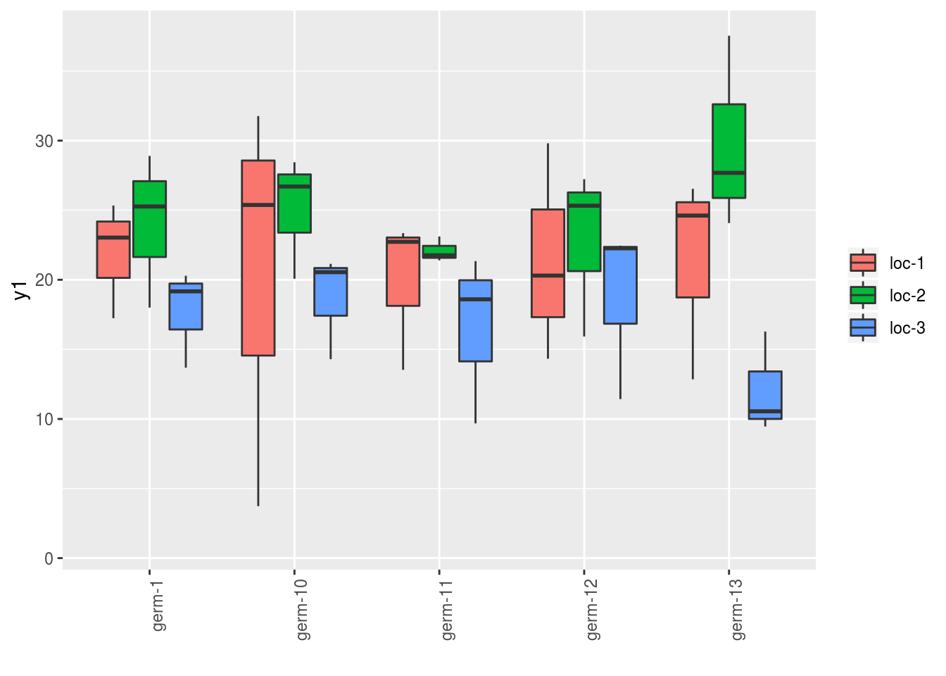

3.4.6 interaction

p = plot(
  data_model_GxE, plot_type = "interaction",
  vec_variables = c("y1", "y2"),
  x_axis = "germplasm",
  in_col = "location"
  )

Note that for each element of the following list, there are as many graph as needed with nb_parameters_per_x_axis and nb_parameters_per_in_col parameters per graph.

names(p$y1)

## [1] "germplasm-1|location-1" "germplasm-2|location-1"
## [3] "germplasm-3|location-1" "germplasm-4|location-1"

p$y1$`germplasm-1|location-1`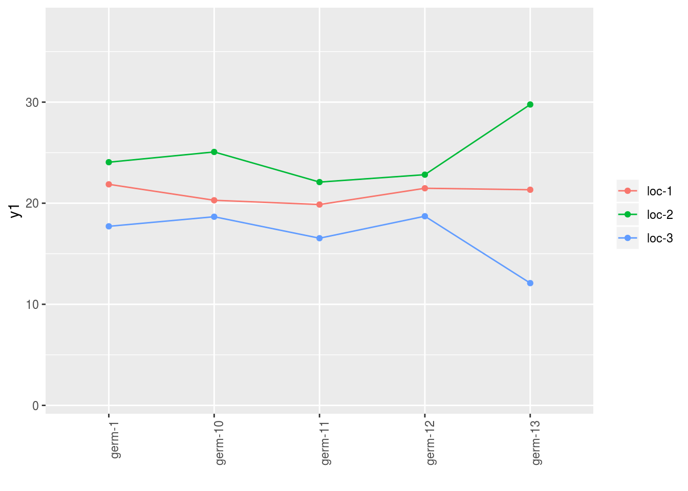

It is also possible to have on the x_axis the date in julian day that have been automatically calculated from format_data_PPBstats(). Note that this is possible only for plot_type = "histogramm", "barplot", "boxplot" and "interaction".

p = plot(
  data_model_GxE, plot_type = "interaction",
  vec_variables = c("y1", "y2"),
  x_axis = "date_julian",
  in_col = "location"
)

## Warning in plot_descriptive_data(x, plot_type, x_axis, in_col,
## vec_variables, : x_axis = "date_julian" is a special feature that will
## display julian day for a given variable automatically calculated from
## format_data_PPBstats().

p$y1$`y1$date_julian-1|location-1`

## geom_path: Each group consists of only one observation. Do you need to
## adjust the group aesthetic?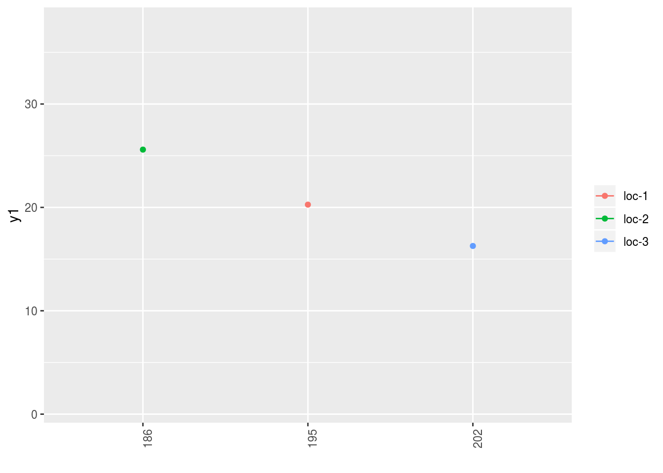

3.4.7 biplot

p = plot(
  data_model_GxE, plot_type = "biplot",
  vec_variables = c("y1", "y2", "y3"),
  in_col = "germplasm", labels_on = "germplasm"
  )

The name of the list correspond to the pairs of variables displayed. Note that for each element of the following list, there are as many graph as needed with nb_parameters_per_in_col parameters per graph.

names(p)

## [1] "y1 - y2" "y1 - y3" "y2 - y3"

p$`y1 - y2`$`-NA|germplasm-1`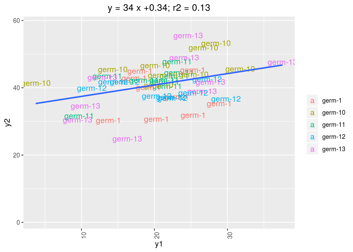

3.4.8 radar

p = plot(
  data_model_GxE, plot_type = "radar",
  vec_variables = c("y1", "y2", "y3"),
  in_col = "location"
  )
p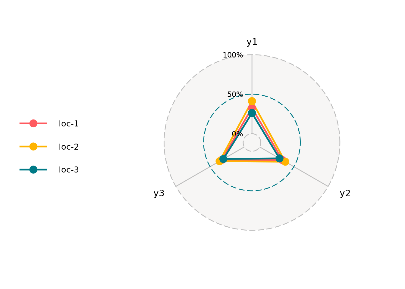

3.4.9 raster

Raster plot can be done for factor variables. Note than when there are no single value for a given x_axis, colums block, X and Y are added in order to have single value.

p = plot(
  data_model_GxE, 
  plot_type = "raster", 
  vec_variables = c("desease", "vigor"), 
  x_axis = "germplasm"
)

## Warning in fun_raster(data, vec_variables, x_axis,
## nb_parameters_per_plot_x_axis): There are no single value for each x_axis,
## therefore block, X and Y colums have been added in order to have single
## value.

p$`germplasm-block-X-Y-9|-NA`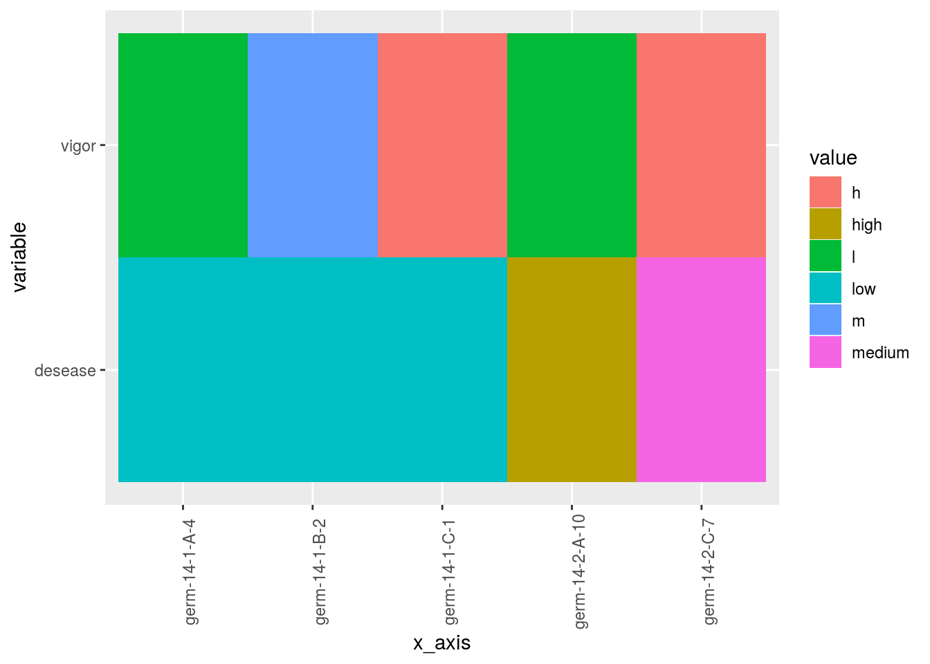

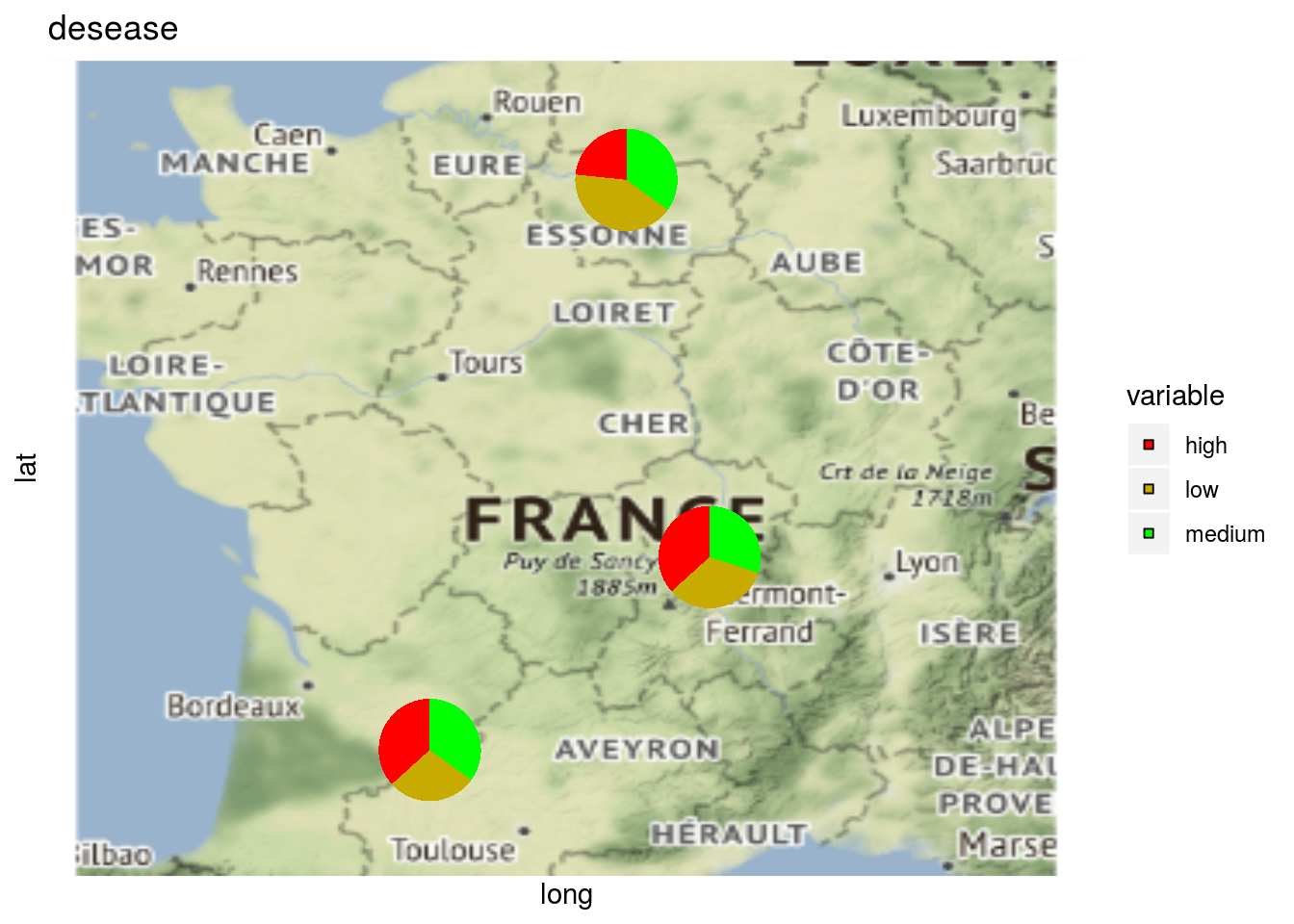
3.4.10 map

You can display map with location if you have data with latitude and longitude for each location. When using map, do not forget to use credit : Map tiles by Stamen Design, under CC BY 3.0. Data by OpenStreetMap, under ODbL.

p = plot(
  data_model_GxE, plot_type = "map", labels_on = "location"
)
p$map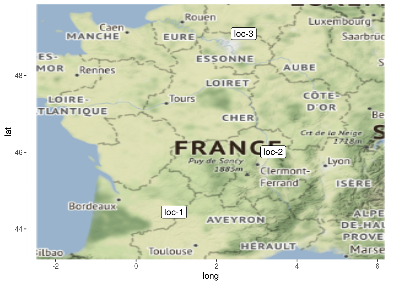

and add pies for a given variables

p = plot(
  data_model_GxE, vec_variables = c("y1", "desease"),
  plot_type = "map"
)
p$pies_on_map_y1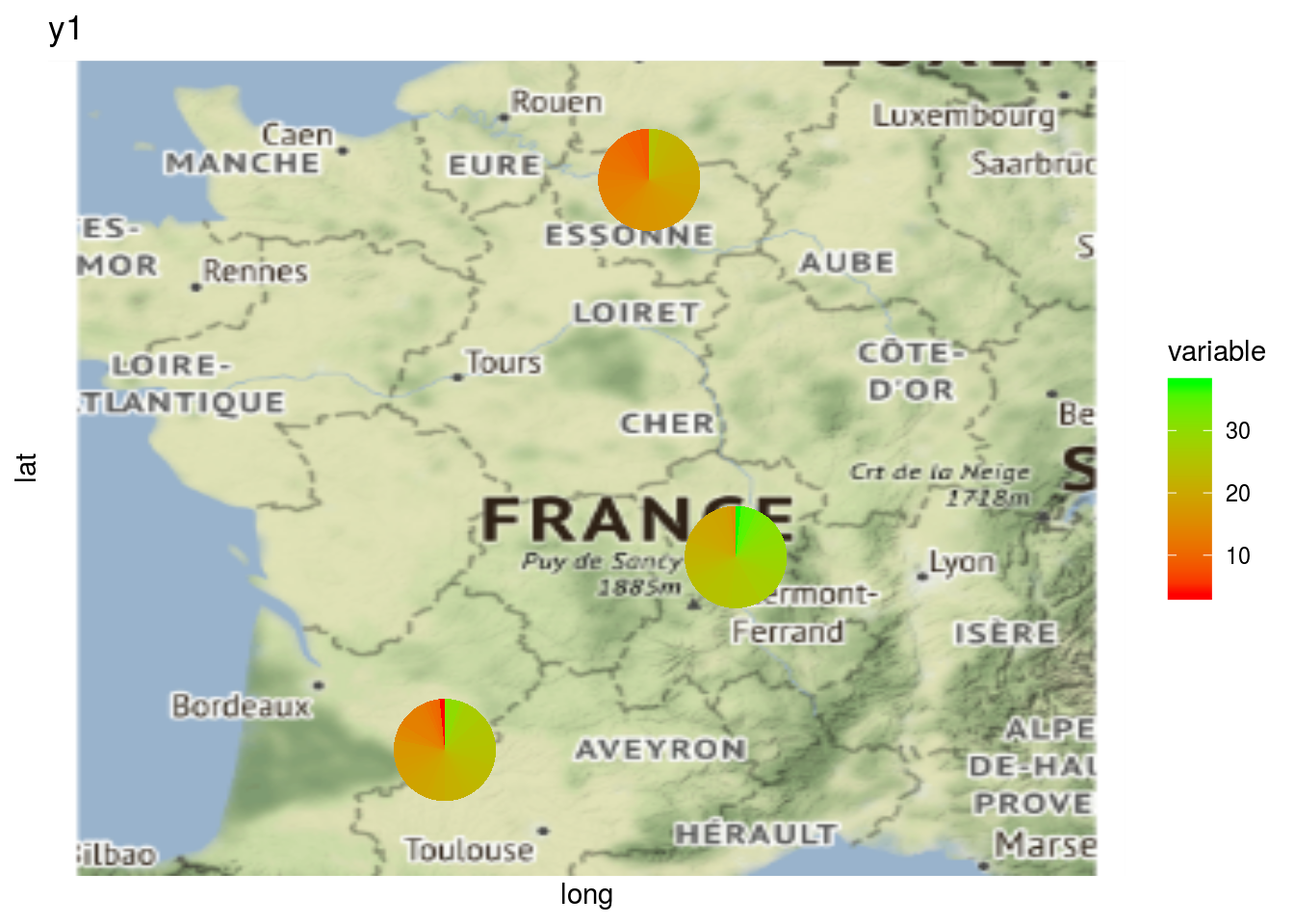

p$pies_on_map_desease