3.1 Introduction
First, chose your objective (3.1.1), then the analyses (3.1.2) and the experimental design (3.1.3) based on a decision tree (3.1.4). Finally see how to implement it based on the workflow and function relations (3.1.5) from formated data (3.1.6).
3.1.1 Analysis according to the objectives
The three main objectives in PPB are to :
- Compare different varieties evaluated for selection in different locations.
This can be done through family 1 of analyses (section 3.5)
- classic anova (M4a, section 3.5.3) based on on fully replicated designs (D1, section 3.2.1),
- spatial analysis (M4b, section 3.5.4) based on row-column designs (D3, section 3.2.3),
- mixed models (M5, section3.5.5) for incomplete blocks designs (D2, section 3.2.2),
- bayesian hierarchical model intra-location (M7a, section 3.5.6) based on satellite-regional farms designs (D4, section 3.2.4).
It can be completed by organoleptic analysis (section 4). Based on these analysis, specific objective including response to selection analysis can also be done.
- Study the response of varieties under selection over several environments.
This can be done through family 2 of analyses (section 3.6):
- AMMI (M6a, section 3.6.3 and GGE (M6b, sections 3.6.4) based on on fully replicated designs (D1, section 3.2.1),
- bayesian hierarchical model \(G \times E\) (M7b, section 3.6.5) based on satellite-regional farms designs (D4, section 3.2.4), It can be completed by specific analysis such as local-foreign (section 3.8.2.3) which corresponds to a specific objective : study local and foreign effect, where foreign in a location refers to a germplasm that has not been grown or selected in a given location and local in a location refers to a germplasm that has been grown or selected in a given location.
- Study diversity structure and identify parents to cross based on either good complementarity or similarity for some traits. This can be done through multivariate analysis and clustering (M2, section 3.9. It can be completed by analysis of molecular data and genetic distance trees (M3, section 5).
3.1.2 Family of analyses
After describing the data (section 3.4), you can run statistical analysis.
Table 3.1 summarizes the analyses available in PPBstats and their specificities.
The various effects that can be estimated are:
- germplasm: a variety or a population
- location: a farm or a station where a trial is carried out
- environment: a combination of a location and a year
- entry: the occurence of a germplasm in a given environment or location
- interaction: interaction between germplasm and location or germplasm and environment
- year
- local-foreign: foreign in a location refers to a germplasm that has not been grown or selected in a given location; local in a location refers to a germplasm that has been grown or selected in a given location.
- version: version within a germplasm, for example selected vs non-selected
The analyses are divided into five families:
Family 1 (section 3.5) gathers analyses that estimate entry effects. It allows to compare different entries on each location and test for significant differences among entries. Specific analysis including response to selection can also be done. The objective to compare different germplasms on each location for selection.
Family 2 (section 3.6) gathers analyses that estimate germplasm and location and interaction effects. This is to analyse the response over a network of locations. Estimation of environment and year effects is possible depending of the model. It allows to study the response of germplasm over several location or environments. The objectives is to study response of different germplasms over several locations for selection.
Family 3 (section 3.7) correspond to combining family 1 and 2 analyses. This allows to analyse network of farms and to study the response of entries over several locations and environnements for selection.
Family 4 (section 3.8) gathers analyses answering specific research questions and objectives such as study intra germplasm variation, study local adaptation with home-away and local-foreign analysis, study differential and response to selection based on models from Family 1.
Family 5 (section 3.9) refers to multivariate analysis
The different models in Family 1 and 2 correspond to experimental designs that are mentionned in the next section 3.1.3 and in the decision tree 3.1.4.
| Family | Name | Section | entry effects | germpasm effects | location effects | environments effects | interaction effects | year effects | local-foreign effects | version effects | variance intra germplasm effects |
|---|---|---|---|---|---|---|---|---|---|---|---|
| 1 | Anova | 3.5.3 | X | ||||||||
| Spatial analysis | 3.5.4 | X | |||||||||
| IBD | 3.2.2 | X | |||||||||
| Bayesian hierarchical model intra-location | 3.5.6 | X | |||||||||
| 2 | IBD | 3.2.2 | X | ||||||||
| AMMI | 3.6.3 | X | X | (X) | X | (X) | |||||
| GGE | 3.6.4 | X | X | (X) | X | (X) | |||||
| Bayesian hierarchical model \(G \times E\) | 3.6.5 | X | X | (X) | X | ||||||
| 3 | Bayesian model 3 | 3.7.1 | X | X | X | X | X | ||||
| 4 | Variance intra | 3.8.3 | X | ||||||||
| Home-away | 3.8.2.2 | X | X | (X) | (X) | (X) | (X) | X | |||
| Local-foreign | 3.8.2.3 | X | X | (X) | (X) | (X) | (X) | X |
Analysis used in PPB programmes are mentionned in decision tree in Section 3.1.4.
3.1.2.1 Frequentist statistics
3.1.2.1.1 Theory
3.1.2.1.2 Check model
Regarding frequentist analysis, there are several ways to check if the model went well.
Residuals distribution. If it looks normal then the hypothesis seems fullfiled.
- Skewness test which is an indicator used in distribution analysis as a sign of asymmetry and deviation from a normal distribution.
- Skewness > 0 - Right skewed distribution - most values are concentrated on left of the mean, with extreme values to the right.
- Skewness < 0 - Left skewed distribution - most values are concentrated on the right of the mean, with extreme values to the left.
- Skewness = 0 - mean = median, the distribution is symmetrical around the mean.
- Kurtosis test which is an indicator used in distribution analysis as a sign of flattening or “peakedness” of a distribution.
- Kurtosis > 3 - Leptokurtic distribution, sharper than a normal distribution, with values concentrated around the mean and thicker tails. This means high probability for extreme values. Kurtosis < 3 - Platykurtic distribution, flatter than a normal distribution with a wider peak. The probability for extreme values is less than for a normal distribution, and the values are wider spread around the mean.
- Kurtosis = 3 - Mesokurtic distribution - normal distribution for example.
Standardized residuals vs theoretical quantiles (qqplot). If the residuals come from a normal distribution the plot should resemble a straight line. A straight line connecting the 1st and 3rd quartiles is added to the plot to aid in visual assessment.
Repartition of variability among factors whici is a pie with repartition of SumSq for each factor. This allows to better understand how the variability is separated between each factor.
- Variance intra germplasm whici is the repartition of the residuals for each germplasm.
With the hypothesis than the micro-environmental variation is equaly distributed on all the individuals (i.e. all the plants), the distribution of each germplasm represent the intra-germplasm variance.
This has to been seen with caution:
- If germplasm have no intra-germplasm variance (i.e. pure line or hybrides) then the distribution of each germplasm represent only the micro-environmental variation.
- If germplasm have intra-germplasm variance (i.e. population such as landraces for example) then the distribution of each germplasm represent the micro-environmental variation plus the intra-germplasm variance.
3.1.2.1.3 Mean comparisons
LSD, LSmeans for home away and local foreign), etc
3.1.2.2 Bayesian statistics
3.1.2.2.1 Theory
Some analyses performed in PPBstats are based on Bayesian statistics.
Bayesian statistics are based on the Bayes theorem:
\(Pr(\theta|y) \propto Pr(\theta) Pr(y|\theta)\)
with \(y\) the observed value, \(\theta\) the parameter to estimate, \(Pr(\theta|y)\) the posterior distribution of the parameter given the data, \(Pr(y|\theta)\) the likelihood of the observation and \(Pr(\theta)\) the prior distribution of the parameter.
The parameters’ distribution, knowing the data (the posterior), is proportional to the distribution of parameters a priori (the prior) \(\times\) the information brought by the data (the likelihood).
The more information (i.e. the larger the data set and the better the model fits the data), the less important is the prior. If the priors equal the posteriors, it means that there is not enough data or the model does not fit the data.
Bayesian inference is based on the posterior distribution of model parameters. This distribution can not be calculated explicitely for the hierarchical model used in here (section 3.5.6 and section 3.6.5) but can be estimated using Markov Chain and Monte Carlo (MCMC) methods.
These methods simulate parameters according to a Markov chain that converges to the posterior distribution of model parameters (Robert 2001).
MCMC methods were implemented using JAGS by the R package rjags that performed Gibbs sampling (Robert 2001).
Two MCMC chains were run independently to test for convergence using the Gelman-Rubin test.
This test was based on the variance within and between the chains (Gelman and Rubin 1992).
A burn-in and lots of iterations were needed in the MCMC procedure. Here the burn-in has 1000 iterations, then 100 000 iterations are done by default5 with a thinning interval of 10 to reduce autocorrelations between samples, so that 10 000 samples are available for inference for each chain by default6 The final distribution of a posterior is the concatenation of the two MCMC chains: 20 000 samples.
3.1.2.2.2 Check model
3.1.2.2.3 Mean comparisons
In this part, the mean of each entry is compared to the mean of each other entry. Let \(H_{0}\) and \(H_{1}\) denote the hypotheses:
\(H_{0} : \mu_{ij} \ge \mu_{i'j} , \; H_{1} : \mu_{ij} < \mu_{i'j}\).
The difference \(\mu_{ij}-\mu_{i'j}\) between the means of entry \(ij\) and entry \(i'j\) in environment \(j\) is considered as significant if either \(H_{0}\) or \(H_{1}\) has a high posterior probability, that is if \(Pr\{H_{0}|y\} > 1 - \alpha\) or \(Pr\{H_{1}|y\}> 1 - \alpha\), where \(\alpha\) is some specified threshold. The difference is considered as not significant otherwise. The posterior probability of a hypothesis is estimated by the proportion of MCMC simulations for which this hypothesis is satisfied (Figure 3.1).
Groups are made based on the probabilites. Entries that belong to the same group are not significantly different. Entries that do not belong to the same group are significantly different.
Note that the term “significant” is not really correct7. Statistical significance refers to the variability of some estimator (e.g. \(\mu_{ij} - \mu_{i'j}\)) under replications of the same experiment (i.e. different datasets), while the posterior probability quantifies the information about some variable given the current dataset. It may be better to claim - based on thershold \(\alpha\) so that whenever the posterior probability of \(H_0\) or \(H_1\) exceeds \(1 - \alpha\) - that the data provides evidence of some difference (not necessarily large) between groups.
The threshold \(\alpha\) depends on agronomic objectives. This threshold is set by default to \(\alpha=0.1/I\) (with \(I\) the number of entries in a given location). It corresponds to a `soft’ Bonferroni correction, the Bonferroni correction being very conservative.
As one objective of this PPB programme is that farmers (re)learn selection methods, the threshold could be adjusted to allow the detection of at least two groups instead of having farmers choose at random. The initial value could be set to \(\alpha=0.1/I\) and if only one group is obtained, then this value could be adjusted to allow the detection of two groups. In this cases, the farmers should be informed that there is a lower degree of confidence for significant differences among entries.
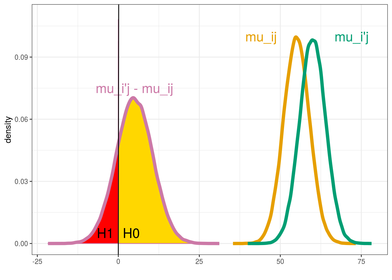
Figure 3.1: Mean comparison between \(\mu_{ij}\) and \(\mu_{i'j}\)
In PPBstats, mean comparisons are done with mean_comparisons.
You can choose on which parameters to run the comparison (parameter argument) and the \(\alpha\) type one error (alpha argument).
The soft Bonferonni correction is applied by default (p.adj argument).
More informations can be obtain on this function by typing ?mean_comparisons.
3.1.3 Experimental design
Before sowing, you must plan the experiment regarding your research question, the amount of seeds available, the number of locations and the number of plots available in each location.
The trial is designed in relation to the analysis you will perform. The key elements to choose an appropriate experimental design are:
- the number of locations
- the number of years
- the replication of entries within and between locations
Several designs used in PPB programmes are mentionned in decision tree in section 3.1.4 and are presented in section 3.2.
3.1.4 Decision tree
For each family of analysis, a decision tree is displayed in the corresponding section. Once you have chosen your objective, analysis and experimental design, you can sow, measure and harvest … (section 3.3).
3.1.5 Workflow and function relations in PPBstats regarding agronomic analysis
After designing the experiment and describing the data, each family of analysis is implemented by several analysis with the same workflow :
- Format the data
- Run the model
- Check the model and visualize outputs
- Compare means and visualize outputs
Note that for some functions for specific model maybe used.
Figure 3.2 displays the functions and their relationships.
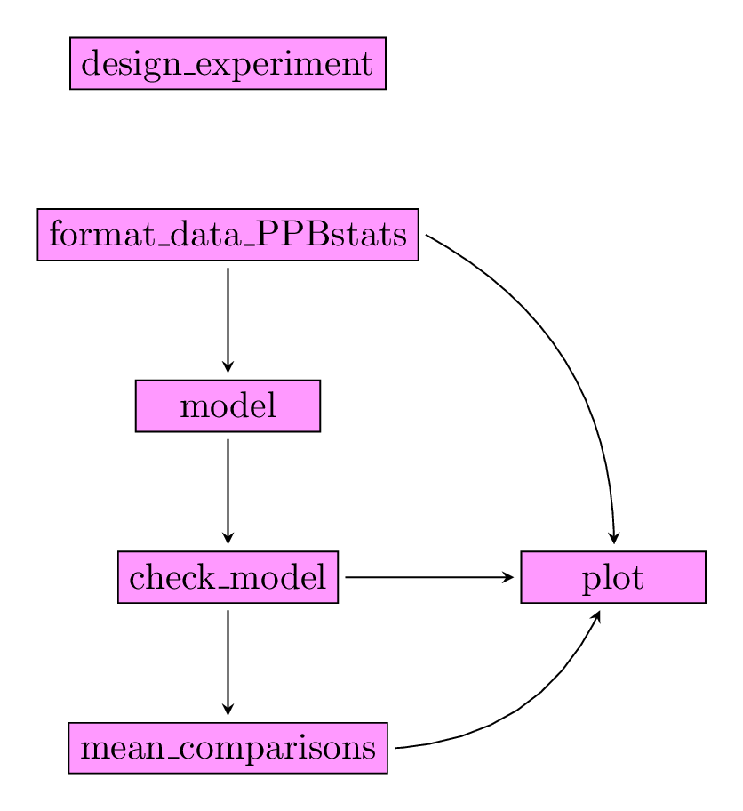
Figure 3.2: Main functions used in the workflow.
3.1.6 Data format
For agronomic analysis data must have a specific format: data_agro
data_agro format corresponds to all the data set used in the functions that run models.
The data have always the following columns : seed_lot, location, year, germplasm, block, X, Y as factors followed by the variables and their corresponding dates.
The dates are associated to their corresponding variable by $.
For example the date associated to variable y1 is y1$date.
In addition, to get map, columns lat and long can be added.
data("data_model_GxE")
data_model_GxE = format_data_PPBstats(data_model_GxE, type = "data_agro")
## data has been formated for PPBstats functions.head(data_model_GxE)## seed_lot location long lat year germplasm block
## 1 germ-12_loc-1_2005_0001 loc-1 0.616363 44.20314 2005 germ-12 1
## 2 germ-1_loc-1_2005_0001 loc-1 0.616363 44.20314 2005 germ-1 1
## 3 germ-18_loc-1_2005_0001 loc-1 0.616363 44.20314 2005 germ-18 1
## 4 germ-14_loc-1_2005_0001 loc-1 0.616363 44.20314 2005 germ-14 1
## 5 germ-6_loc-1_2005_0001 loc-1 0.616363 44.20314 2005 germ-6 1
## 6 germ-4_loc-1_2005_0001 loc-1 0.616363 44.20314 2005 germ-4 1
## X Y y1 y1$date y2 y2$date y3 y3$date desease
## 1 A 1 14.32724 2017-07-15 41.85377 2017-07-15 66.05498 2017-07-15 low
## 2 A 2 23.03428 2017-07-15 37.38970 2017-07-15 63.39528 2017-07-15 low
## 3 A 3 24.91349 2017-07-15 38.38628 2017-07-15 60.52710 2017-07-15 high
## 4 A 4 24.99078 2017-07-15 39.72205 2017-07-15 60.80393 2017-07-15 low
## 5 A 5 18.95340 2017-07-15 46.60443 2017-07-15 53.71210 2017-07-15 high
## 6 B 1 21.31660 2017-07-15 49.94656 2017-07-15 60.71978 2017-07-15 medium
## vigor y1$date_julian y2$date_julian y3$date_julian
## 1 l 195 195 195
## 2 l 195 195 195
## 3 h 195 195 195
## 4 l 195 195 195
## 5 m 195 195 195
## 6 l 195 195 195Note that a column with julian date is added.
class(data_model_GxE)## [1] "PPBstats" "data_agro" "data.frame"Note that other formats exist in relation to specific reasearch questions as explained in section 3.8.
References
Gelman, A., and D.B. Rubin. 1992. “Inference from Iterative Simulation Using Multiple Sequences (with Discussion).” Statistical Science, no. 7: 457–511.
Robert, C.P. 2001. The Bayesian Choice. Second. Springer Texts in Statistics. Springer.